6. Jádrová regrese Lineární expanze do bázových funkcí, duální formulace, jádrový trik

Recap

Linear Regression

Linear Regression is a supervised machine learning algorithm where the predicted output is continuous and has a constant slope. It is used to predict values within a continuous range, (for instance, predicting house prices based on various features like area, number of rooms, etc.) rather than trying to classify them into categories.

The linear regression model is represented as: $Y = w_0 + w_1x_1 + ... + w_px_p + \varepsilon$

Here,

• $Y$ is the target variable,
• $x_1,..., x_p$ are features,
• $w_0,..., w_p$ are weights or coefficients,
• $\varepsilon$ is the error term.

Our aim is to estimate the unknown vector $w$.

The training model is written in a matrix form as $Y = Xw + \varepsilon$. Here $X$ is the feature matrix and $\varepsilon$ is a vector of error terms.

Ordinary Least Squares

Ordinary least squares (OLS) is a method for estimating the unknown parameters in a linear regression model. OLS chooses the parameters of a linear function of a set of explanatory variables by the principle of least squares: minimizing the sum of the squares of the differences between the observed dependent variable in the given dataset and those predicted by the linear function.

The solution of the normal equations $X^TY - X^TXw = 0$ , which correspond to the gradient of the residual sum of squares is $\hat{w} = (X^TX)^{-1}X^TY$.

Ridge Regression

Ridge regression is a regularization technique used when the predictors in a regression are highly correlated (multicollinearity). By shrinking the coefficients of the predictors, Ridge regression reduces model complexity and multicollinearity. This is commonly used in situations where we have many variables contributing to a prediction, like predicting consumer behavior based on various characteristics.

The Ridge regression minimizes the regularized residual sum of squares given by:

$RSS_{\lambda}(w) = ||Y − Xw||^2 + \lambda\sum_i(w_i)^2$

Here $\lambda \geq 0$ is a complexity parameter that controls the amount of shrinkage: the larger the value of $\lambda$, the greater the amount of shrinkage.

Linear Expansion into Basis Functions

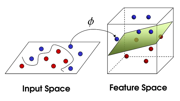
In the context of kernel regression, the relationship between $x$ and $y$ is modelled through basis functions, $\phi(x)$, which transform the input data $x$ into a higher dimensional feature space. This allows the model to capture more complex, nonlinear relationships. For example, this concept can be used in image recognition where the features extracted from an image are transformed into a higher-dimensional space.

The transformation looks like this:

$$f(x) =\varepsilon + \sum_{i=1}^{d} w_i*\phi_i(x)$$

Here, $\phi_i(x)$ are the basis functions and $w_i$ are the weights for each basis function.

Dual Formulation

Many linear models for regression and classification may be formulated in terms of a dual representation where the basis functions ($\phi(x)$) are given implicitly through the so-called kernel function where kernel functions are $k(\mathbf{x}_i, \mathbf{x}_j)$.

Key points 1. The dual version of the regularized residual sum of squares is minimized, which is given by: $$\text{RSS}_{\lambda}(\alpha) = \|\mathbf{Y} - \mathbf{G}\alpha\|^2 + \lambda \alpha^T \mathbf{G}\alpha$$ where $G_{i,j} = k(\mathbf{x}_i, \mathbf{x}_j)$ and gram matrix $G=\Phi\Phi^T$

1. The minimizer, for any $\lambda > 0$, is given by: $$\hat{\alpha} = (\mathbf{G} + \lambda\mathbf{I})^{-1}\mathbf{Y}.$$
2. Prediction of Y at any point x is then: $$\hat{Y} = \sum_{i=1}^{N} \hat{\alpha}_i k(\mathbf{x}_i, \mathbf{x}) = \hat{\alpha}^T k(\mathbf{x}).$$

Or in other way in the dual formulation, instead of finding a direct mapping of $x$ to $Y$, we find a mapping of $x$ to $Y$ via a higher dimensional space $z$. This can be written as:

$$f(x) = \sum_{i=1}^{n} \alpha_i*y_i*k(x_i, x) = \hat{\alpha}k(x)$$

where $k(x_i, x)$ is a kernel function which computes the inner product of $x$ and $x_i$ in the feature space, and $\alpha_i$ are the dual coefficients. Therefore not only the objective function $\text{RSS}_{\lambda}(\alpha)$ but also the predictions $\hat{Y}$ might be expressed entirely in terms of the kernel function $k$.

Kernel Trick

Further reading The kernel trick is a method used in machine learning to transform the input data into a high-dimensional feature space, where complex relationships can be modeled using simpler, linear models. Instead of explicitly calculating the transformation $\phi(x)$, we use a kernel function $K(x, x_i) = \phi(x)^T*\phi(x_i)$. This is especially useful in problems where the data is not linearly separable in the input space but might be in a higher-dimensional space.

Key points

1. The kernel trick allows the input vector to enter the model only in the form of scalar products, leading to an equivalent dual representation of the model along with the objective function.

2. By not explicitly specifying the basis functions, the kernel trick permits the implicit use of feature spaces with high, even infinite, dimensionality.

3. The computational advantage comes into play when dealing with high-dimensional spaces as the matrix inversion required in the estimation of weights and $\alpha$ has complexity $O(M^3)$ and $O(N^3)$, respectively. Where, $M$ is the dimensionality of the feature space and $N$ is the number of data points.

   1. An application of the kernel trick would be in regression over large datasets, such as $1000$ gray scale images of $32 \times 32 = 1024$ pixels. For instance, using a quadratic kernel $k(\mathbf{x}, \mathbf{y}) = (\mathbf{x}^T \mathbf{y}+1)^2$, we would expand into a $525,825$ dimensional space. Despite the high dimensionality, the inversion of only a $1000 \times 1000$ matrix is required, instead of a $525,825 \times 525,825$ matrix, illustrating the power of the kernel trick.

Key Takeaways

• Kernel Regression: Kernel regression is a non-parametric technique that allows the data to determine the form of the function $f(x)$. This makes it highly flexible and capable of modeling complex relationships.

• Linear Expansion into Basis Functions: This involves transforming the input data $x$ into a higher dimensional feature space using basis functions $\phi(x)$. This allows the model to capture more complex, potentially non-linear relationships.

• Dual Formulation: In the dual formulation, we find a mapping from $x$ to $y$ via a higher dimensional space $z$. This is a key concept in many machine learning models.

• Kernel Trick: The kernel trick allows us to compute the inner products in the high-dimensional space without explicitly calculating the transformation $\phi(x)$, making the computation significantly simpler and more efficient.