EDA CARD TRANSACTIONS AT PETROL STATIONS

About

This dataset contains card transactions made by clients of some small Czech bank at petrol stations, mostly in the Czech republic but also abroad, in the period of 12 months in 2017-2018.

Columns

• clid: client id
• posid: id of the payment place (petrol station)
• day: payment date in the Y-m-d format
• hour: payment hour (0-23)
• amt: payment amount in CZK
• fav: is this station flagged to be one of favourite stations of that client?
• fav_main: is this station flagged to be the most favourite station of that client?
• cl_gps_lat, cl_gps_lon: GPS coordinates of the client's living place (possibly the municipality only, not street or house exactly)
• country: payment country
• city: payment city
• name: payment place (station) name
• clst: number of cluster where the station fits by clients behaviour (0 = unclustered)
• pos_gps_lat, pos_gps_lon: GPS coordinates of the payment place (for the stations in the Czech republic only)
• dist: distance in km between client living place and payment place

Problem Statement

Our objective is to forecast the following attributes for a user's subsequent visit to a gas station:

• Time: When will the user visit next?
• Location: Which gas station (specified by its coordinates, address or other location marker ) will the user choose for their next visit?
• Transaction Amount: How much will the user spend during their next visit?

General analysis

The aim is to find answers to questions:

• How many rows are there? What does represent each rows? Do we need any aggregation or reshaping? Are all rows useful for our purpose? Do we need to make a sample? Does each row have its unique ID?
• How many columns are there? What are their names, types, meanings?
• Are there any duplicated rows (with exclusion of ID)?
• What are counts and shares of missing values in the dataset columns?
• Are counts of missing values expectable and acceptable?
• Are any columns or rows (almost) empty and may be removed as useless?

Summary: What initial transformations of the dataset are useful or necessary?

General Analysis Summary:

1. Duplicate Rows:
2. Observation: There are some rows in the dataset that are duplicates.

3. Action: These duplicate rows can be removed to maintain data integrity and avoid redundancy in analysis.

4. Missing Point of Sale Coordinates (pos_gps_lat & pos_gps_lon):

5. Observation: A significant number of transactions are missing their Point of Sale GPS coordinates.

6. Action: We can compute or approximate these values using the available 'country' and 'city' columns. This would provide a general idea of the transaction location, even if it's not precise.

7. Distance (dist):

8. Observation: Some entries are missing distance values.

9. Action: We can roughly estimate the distance using the computed/approximated Point of Sale GPS coordinates and the client's coordinates.

10. Client Coordinates (cl_gps_lat & cl_gps_lon):

11. Observation: A small fraction of transactions is missing client GPS coordinates.

12. Action: Given the small proportion of these missing values compared to the dataset's size, they can be removed without significantly impacting the analysis.

13. Country & City:

14. Observation: There are a few transactions with missing 'country' and 'city' values.
15. Action: As with the client coordinates, given their small proportion, these rows can be safely removed.

Distributions of individual variables

The aim is, for each column individually, to find answers to questions:

• Are values plausible?
• Are there any values standing for missing (NA), empty or other special cases?
• Is type of column appropriate for its values? Should we change it?
• How should we treat missing values?
• Numerical: How should we treat outliers?
• Numerical: Could/should we make a binning (and if so, how)?
• Categorical: Which categories could be joined?
• What is distribution of values? What does it mean for the problem we try to solve?

Summary: In which columns should we consider fixing of values (correction, filling, replacing etc.) or transformation of them (type change, recalculating, binning etc.)? What story do data tell us? What could/should we explore more deeply?

Distributions of individual variables summary:

Column Name	Observations & Plausibility	Action
clid, posid	Values seem plausible as IDs. No missing values.	Do not use in ML models.
day	Values seem plausible as valid dates. No missing values.	Split into: day of the week, month, actual day, and season for ML use.
hour	Values seem plausible as hours. Some missing values.	Suitable in current format. Delete missing values.
amt	Values seem plausible as transaction amounts. No missing values and no negative values detected.	Suitable in current format.
fav, fav_main	Binary representation with values 0 or 1. No missing values and no other values then 0 and 1.	Suitable in current format.
cl_gps_lat, cl_gps_lon	Values within latitude and longitude ranges. Missing values present.	Remove rows with missing GPS data. Convert into zone data for ML models.
country, city	Valid country and city names observed. Few missing entries detected.	Remove rows with missing country, city, and GPS data.
name	Represents transaction entities. No missing values.	Suitable in current format. Use encoding strategies in ML models.
clst	Category representation observed. Value "0" indicates unclustered. Significant missing values present.	Missing values add into a new category. Treat as categorical for ML models.
pos_gps_lat pos_gps_lon	Valid latitude and longitude ranges observed. Significant missing values present.	Derive or approximate based on the country and city columns. Delete rows if both city and country data are missing. Convert into zone data for ML models.
dist	Distances observed are non-negative. Significant missing values present.	Compute from GPS data. Delete rows where computation is not feasible.
## Exploratory data analysis

• distribution of clients by number of payments, number of distinct stations, average amount etc.
• distribution of amounts and relationship to season, hour, day in month etc.
• distribution of stations by number of payments, number of distinct clients, average amount etc.
• distribution of distance client-station, relationship to season, hour, day etc.
• distribution of payments during a day, a week, a month
• trends (time series) of payment number, amount etc.
• distribution of stations in the Czech Republic, highway twins (stations on opposite sides of highways) similarity/dissimilarity
• favourite station brands

Clients

The dataset provides insights into client behaviors regarding their transactions at gas stations. One way to understand these behaviors is by analyzing the distribution of their transactions and the variety of gas stations they visit.

Distribution of clients by number of payments

The number of payments made by a client can give insights into their frequency of visits to gas stations. It may be indicative of their travel habits, vehicle usage, or even loyalty to specific gas brands.

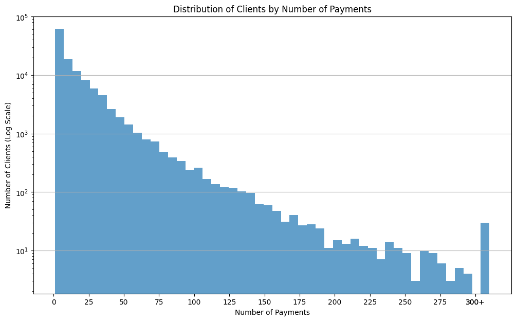
From the histogram, we observe that a majority of clients have made a smaller number of payments, suggesting infrequent visits or usage. However, a small proportion of clients have a significantly higher number of transactions, indicating more regular visits or potentially commercial usage.

Distribution of clients by number of visited unique gas stations

Exploring the number of unique gas stations visited by clients can provide insights into their brand loyalty or their travel patterns.

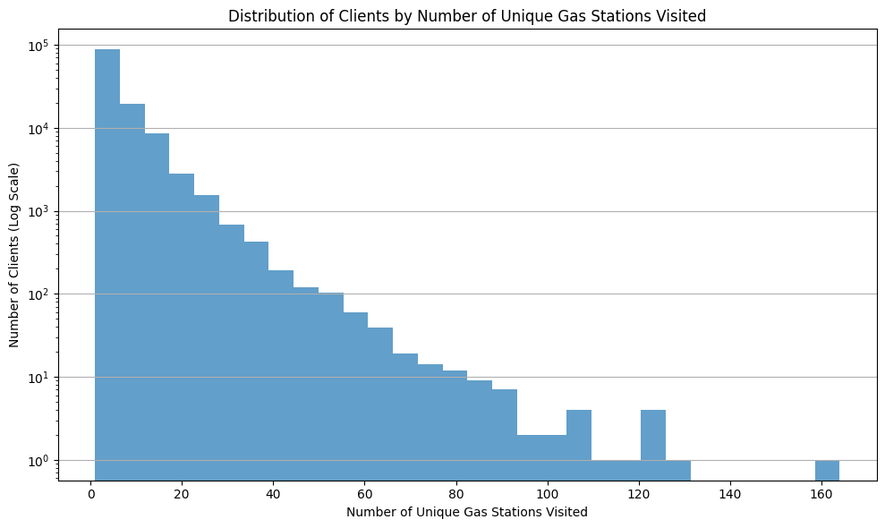
The histogram suggests that many clients stick to a limited set of gas stations, possibly indicating brand loyalty or localized travel patterns. Fewer clients have visited a broader range of stations, suggesting more extensive travel or lesser brand loyalty which could be commercial user like truckers.

Correlation between number of payments and number of visited unique gas stations

Understanding the relationship between the number of payments and the variety of gas stations can provide insights into client behaviors.

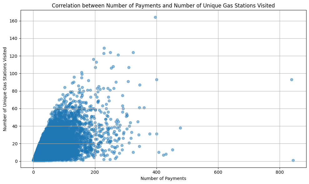
Correlation between the number of payments and number of unique gas stations visited 0.74

The scatter plot and the calculated Pearson correlation coefficient indicate a positive relationship. Clients who visit more unique gas stations also tend to make more payments, suggesting that diversified visits might be associated with higher usage or travel frequencies and tendency for larger clients not having brand loyalty.

Correlation between number of payments and number of unique gas stations brands visited

Exploring the correlation between the number of payments and the variety of gas station brands can offer insights into brand loyalty. Do clients who refuel frequently tend to stick to specific brands, or are they open to trying different ones? As previously hinted by the previous correlation.

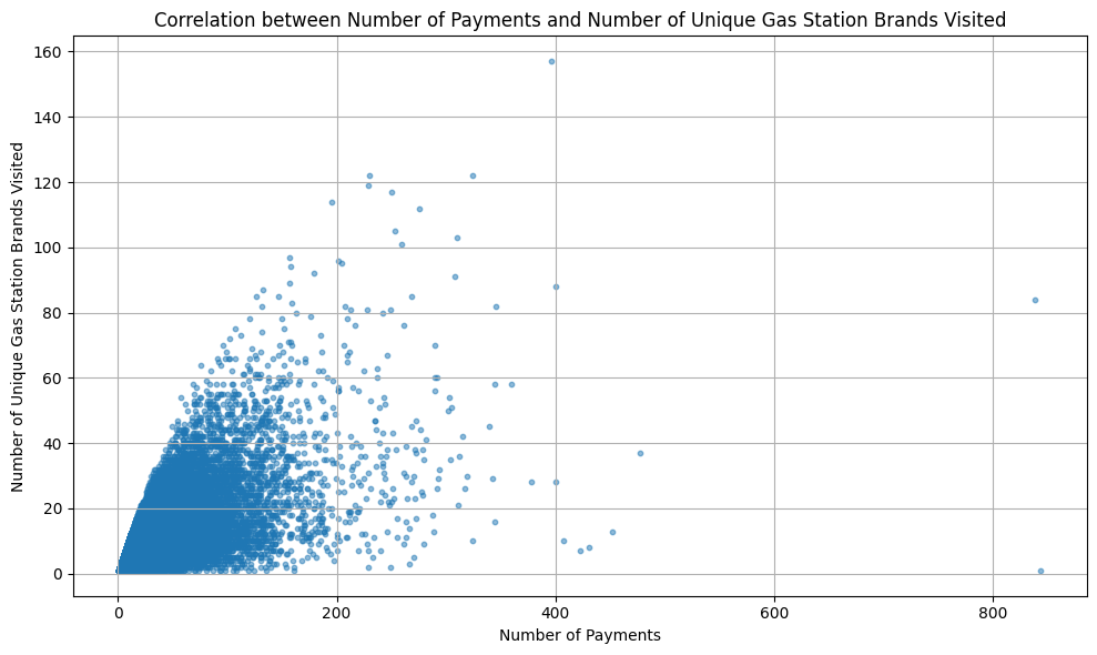
Correlation between the number of payments and number of unique gas stations brands visited 0.739

The scatter plot highlights a positive trend. Clients who have made more payments also seem to have experienced a diverse range of gas station brands. This could be indicative of non-loyal behavior, suggesting that promotions or brand-specific loyalty programs might not be as effective for these high-frequency clients.

Distribution of distances clients travel to refuel

This will provide insights into how far clients are typically willing to travel.

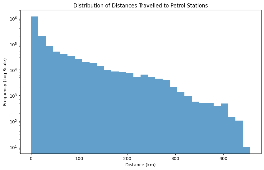
The histogram indicates that a significant number of clients tend to refuel at stations that are relatively close to their residences

Correlation Between 'Favorite' and Transaction Amounts or Frequency

We'll now investigate if transactions at stations flagged as 'favorite' have different characteristics in terms of transaction amounts and frequency compared to those at non-favorite stations.

Favourite Station Analysis Results:

1. Transaction Frequency:
   - Non-Favorite Stations (Favorite = 0): 841,476 transactions
   - Favorite Stations (Favorite = 1): 1,012,075 transactions
2. Average Transaction Amount:
   - Non-Favorite Stations (Favorite = 0): 542.82 CZK
   - Favorite Stations (Favorite = 1): 558.12 CZK
3. Median Transaction Amount:
   - Non-Favorite Stations (Favorite = 0): 384.00 CZK
   - Favorite Stations (Favorite = 1): 406.00 CZK

Flagging a station as 'favorite' does show a correlation with both increased transaction amounts and frequency, though the difference isn't substantial. Clients appear to have a slight preference for their favorite stations, visiting them marginally more often and spending a bit more during each visit compared to non-favorite stations.

Payment Amount

In this section, we'll focus on the payment data. We'll explore the distribution of transaction amounts, understand when and where these payments are higher or lower, and identify patterns related to spending at petrol stations. This will give us insights into customer behaviors and station preferences.

Distribution of Transaction Amounts at Petrol Stations

This histogram provides an overview of the range and frequency of transaction amounts.

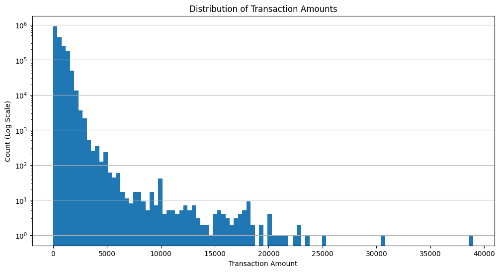
It's evident that smaller transaction amounts are more common, with a few larger transactions interspersed. Again showing that the dataset contains users diverging from the norm.

Monthly Variation in Transaction Amounts

Understanding monthly variations in transaction amounts is crucial for petrol stations. By examining how transaction amounts change month-to-month, stations can anticipate trends, manage inventory effectively, and tailor promotions to maximize revenue.

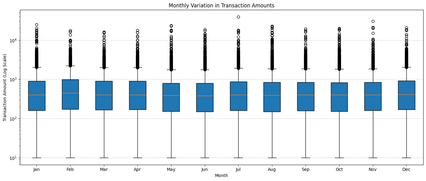
The monthly breakdown reveals consistent median transaction amounts, suggesting a regular spending pattern by customers throughout the year.

Weekly Variation in Transaction Amounts

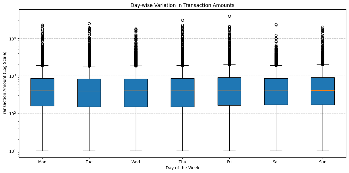
The day-wise distribution reveals a consistent median transaction amount throughout the week.

Daily Variation in Transaction Amounts

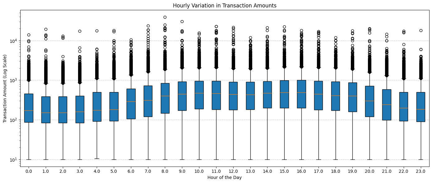
The hourly distribution of transaction amounts reveals notable patterns. Specifically, there's an evident trend of increased spending between the hours of 8 and 19

Payment frequency

We'll continue to focus on the payment data but this time its frequency. We'll explore the distribution of transaction frequency, understand when and where these payments are more or less frequent, and identify patterns related to frequency at petrol stations. This will give us insights into customer behaviors and station preferences.

Monthly Payment Frequency

We'll explore how often payments are made in each month to understand if there are specific months where transactions are more frequent.

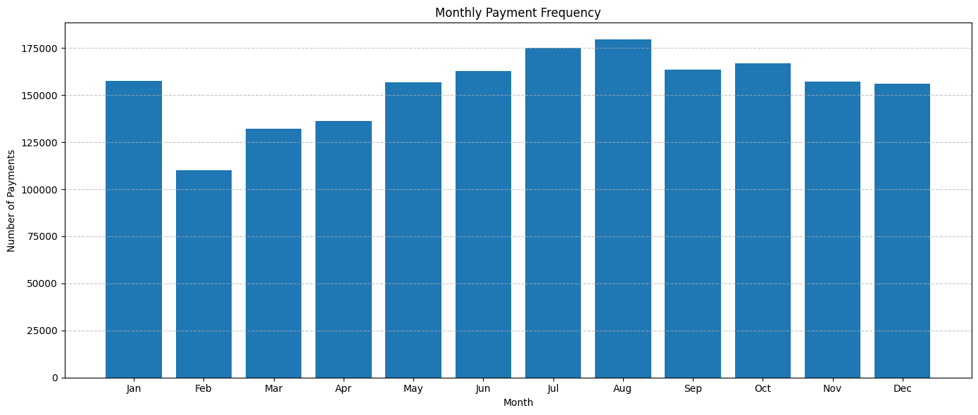
Starting in February, there's a noticeable decline in gas station transactions. This dip is followed by a steady rise, peaking in July and August. After these summer months, the transaction frequency remains consistent through to the end of the year. However, as we transition from January to February, there's another noticeable drop in transactions.

This pattern could be attributed to several factors. The decline in February might be linked to post-holiday financial adjustments, as consumers might be more frugal after the often expensive holiday season in December. The increase leading up to and peaking in the summer months could be due to vacation travel, with more people hitting the roads for holidays and trips. The stability observed from August to January might reflect regular commuting and travel behaviors.

But, as we observed, the payment amount doesn't vary significantly, implying that the transaction value remains consistent. This suggests that only a portion of the population is able to economize on gas and adopt a more frugal approach. Meanwhile, a significant number of users either can't or choose not to alter their habits. This could be indicative of essential travel needs, where certain segments of the population have non-negotiable commuting or travel requirements, regardless of the season or economic factors.

Weekly Payment Frequency

Next, we'll delve into the weekly distribution to discern which days of the week witness higher transaction frequencies. This will provide insights into potential peak days for petrol stations.

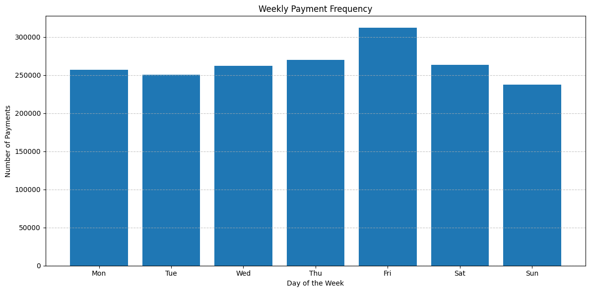
Examining the transactions on a weekly basis, the frequency of payments is relatively consistent for most days. However, an exception is observed on Friday, where there's a noticeable uptick in the number of transactions. This surge is followed by a decline on Saturday and Sunday, bringing the transaction frequency back to the levels seen during the earlier part of the week.

The heightened activity on Friday could be attributed to several factors. Some people might be refueling in anticipation of weekend travels or outings. Additionally, for those who get paid on Fridays, it might be a convenient day to fill up their tanks. The subsequent drop over the weekend could indicate that a significant portion of the population completes their refueling needs by Friday, reducing the necessity for weekend and weekday visits to the gas station.

Hourly Payment Frequency

To further refine our understanding, we'll now evaluate the hourly distribution. Knowing the times of day when transactions are most frequent can aid petrol stations in optimizing their operations for peak hours.

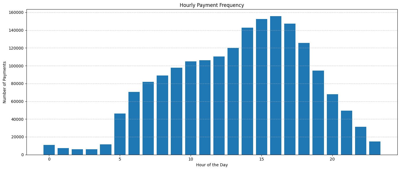
On an hourly basis, the payment frequency reveals a clear pattern. From 10 PM until 4 AM, there's a significant drop in card transactions, indicating that these are the quietest hours for gas stations. Beginning at 5 AM, there's a noticeable increase in transactions, which steadily rises throughout the morning and afternoon, reaching its peak around 5 PM. After this high point, the frequency starts to decline steadily, continuing until 10 PM.

This trend likely mirrors typical daily routines. The early morning uptick in transactions could be attributed to commuters refueling their vehicles before heading to work. The peak in the late afternoon might be associated with individuals refueling on their way home from work. The subsequent decline in the evening and the minimal transactions during the late-night hours suggest that fewer individuals are on the roads, leading to reduced transactions at petrol stations during these times.

Time series analysis of transaction rates

Diving deeper into our data, a time series analysis is essential to further understand the transaction rates at petrol stations. This approach will help us track transaction trends over time, enhancing our understanding of observed patterns like the notable monthly variations and distinct hourly behaviors. For instance, while we've seen consistent weekly transactions with a spike on Fridays and quieter late-night hours, a time series analysis will validate if these trends persist over longer durations. Through this, petrol stations can better plan for recurring busy periods, adapt to quieter times, and align their services with established customer patterns.

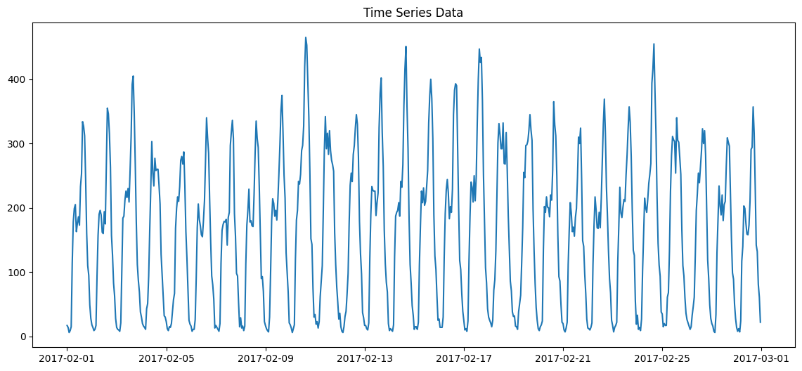
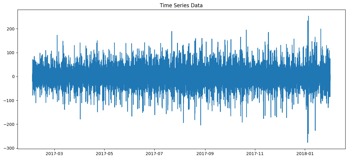
Initial visualisation

The first step in any time series analysis is to visualize the data. This gives us a preliminary understanding of any visible trends, patterns, or anomalies in the data.

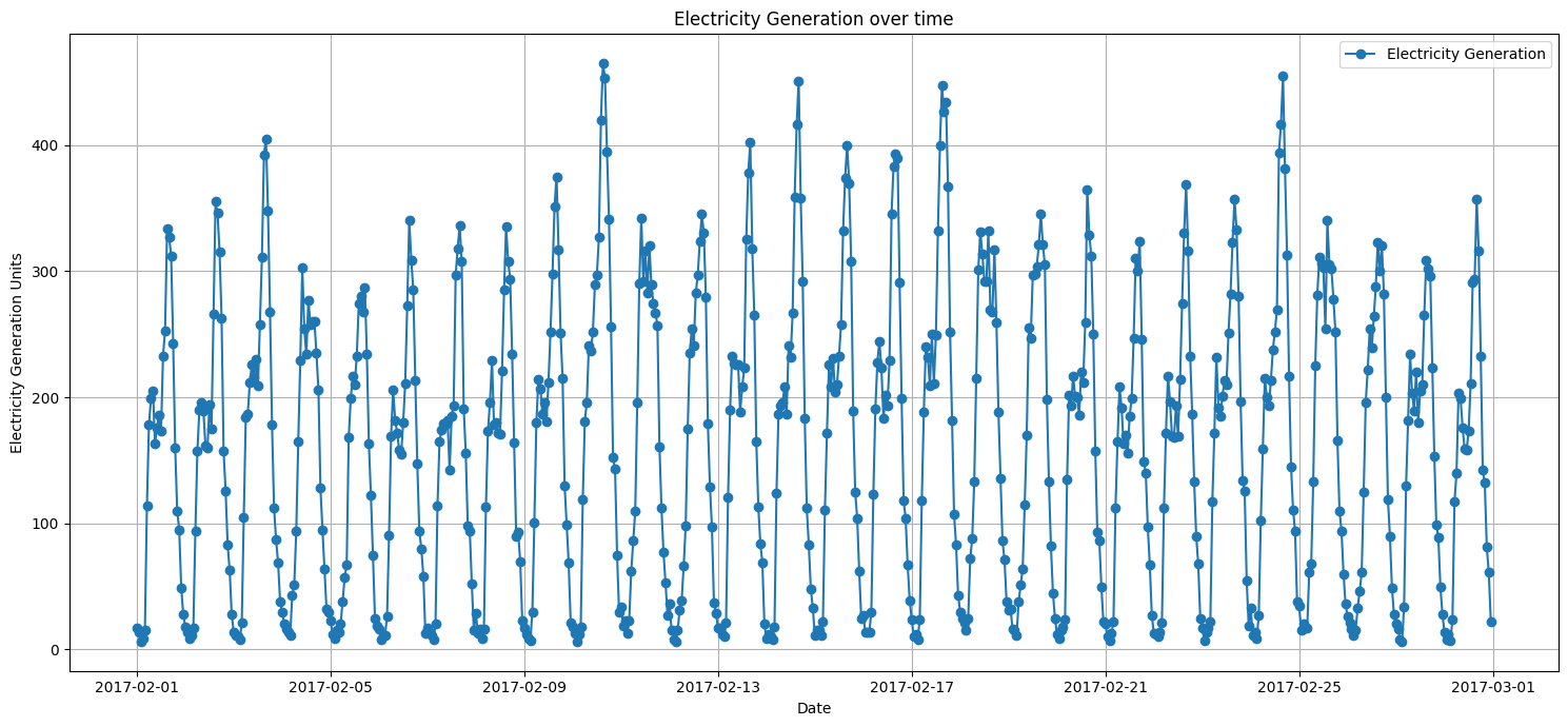
From the initial visualization, we can observe daily patterns. The transaction rate seems to have regular peaks and valleys, suggesting daily seasonality. Which is not unexpected given our previous analysis

Initial decomposition

Decomposing the time series will further help in understanding its underlying structure by splitting it into three components: trend, seasonality, and residuals.

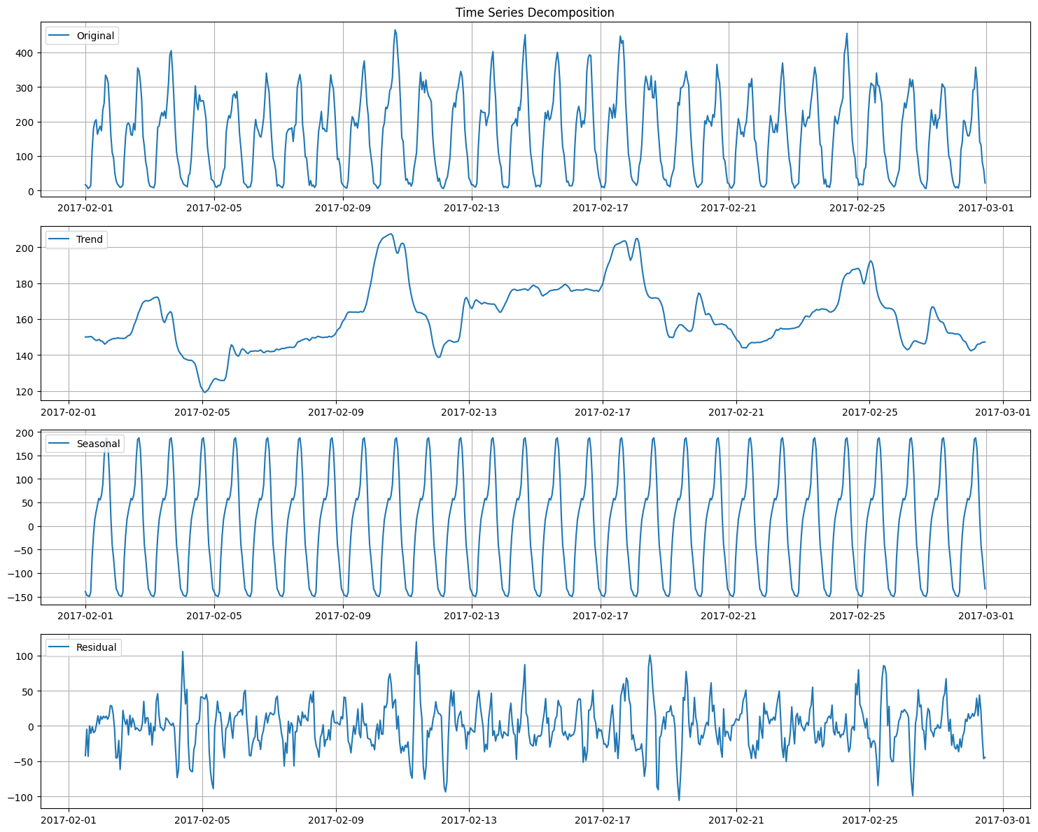
As expected, the decomposition confirms the daily seasonality we observed in the initial visualization. But we can still see weekly seasonality which again is not unexpected. So lets try the weekly seasonality

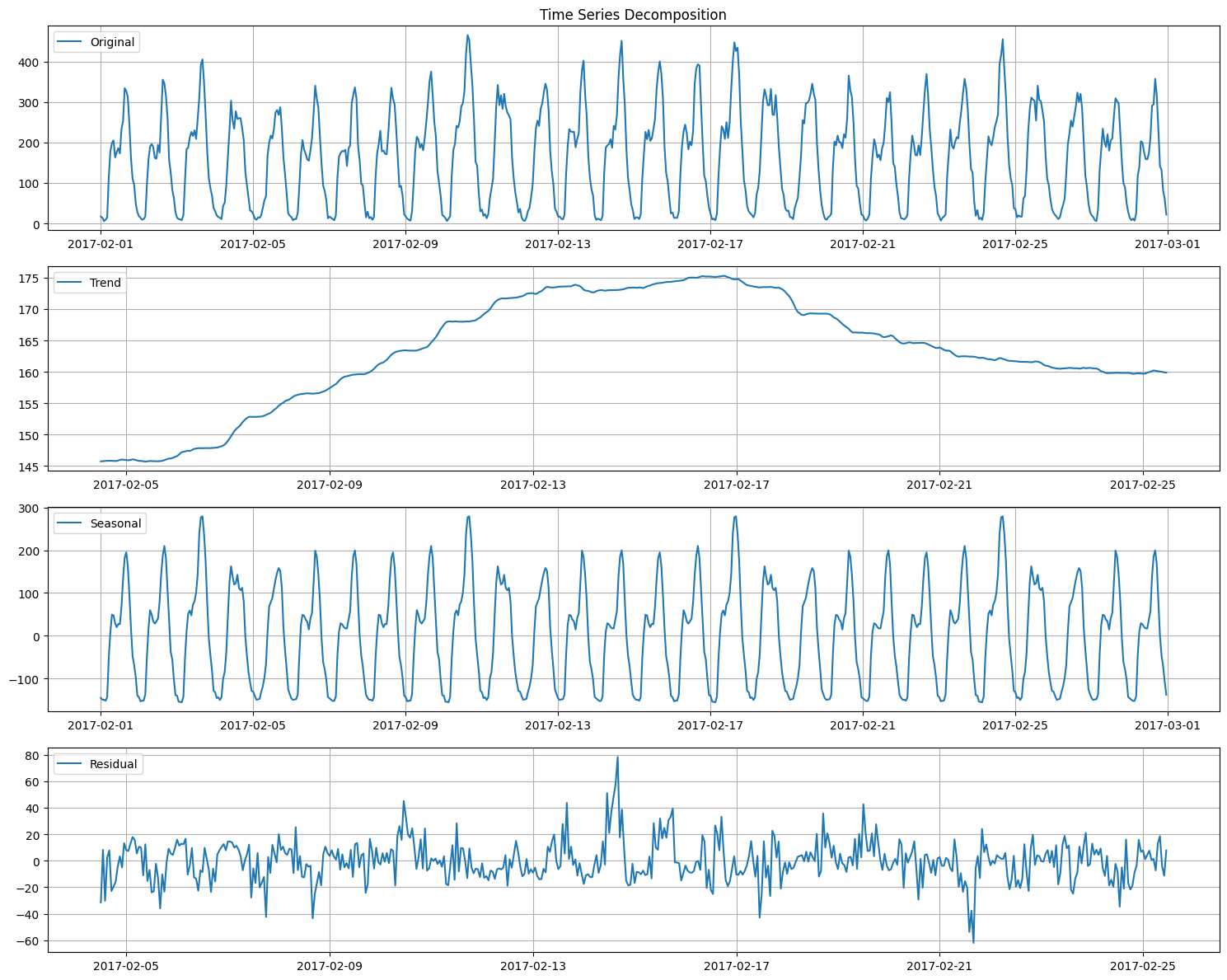
The trend component is finally relatively stable over this short duration, and the residuals don't show any significant pattern, which is a good sign.

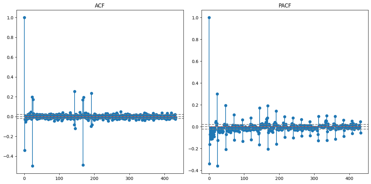
Autocorrelation

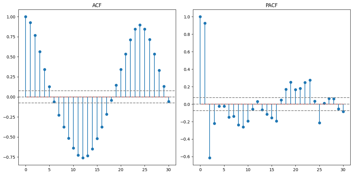
The ACF plot will help identify any autocorrelation in the data. If our hypothesis of a 24-hour seasonality is correct, the ACF plot should show significant spikes at lag values of 24, 48, etc.

ADF Test:
----------------------------------------
ADF Statistic: -4.2631
p-value: 0.0005
Critical Value 1%: -3.4404
Critical Value 5%: -2.8660
Critical Value 10%: -2.5691
----------------------------------------

KPSS Test:
----------------------------------------
KPSS Statistic: 0.0799
p-value: 0.1000
Critical Value 10%: 0.3470
Critical Value 5%: 0.4630
Critical Value 2.5%: 0.5740
Critical Value 1%: 0.7390
----------------------------------------

Stationarity Assessment:
The time series is stationary.

Indeed, the ACF confirms the 24-hour seasonality. There's a strong autocorrelation at a lag of 24 hours. The function also tells us that the time series is not stationary

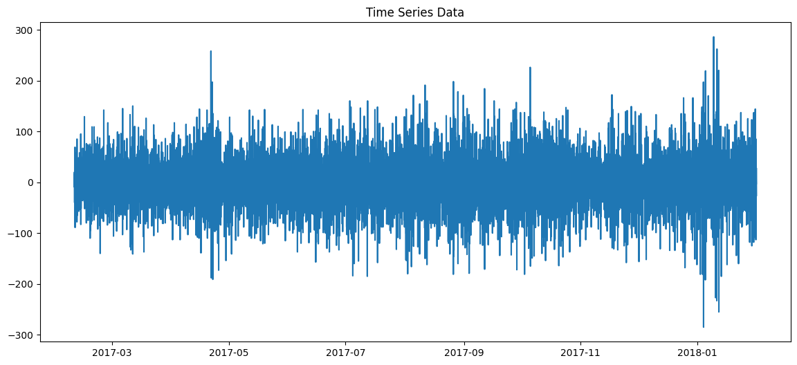
• First-order differencing
  • We'll apply first-order differencing to the time series and analyze its properties.
• Seasonal differencing
  • To address the 24-hour seasonality, we apply a seasonal difference, which is the difference between an observation and the previous observation from the same time of day.

ADF Test:
----------------------------------------
ADF Statistic: -24.4669
p-value: 0.0000
Critical Value 1%: -3.4311
Critical Value 5%: -2.8619
Critical Value 10%: -2.5669
----------------------------------------

KPSS Test:
----------------------------------------
KPSS Statistic: 0.0106
p-value: 0.1000
Critical Value 10%: 0.3470
Critical Value 5%: 0.4630
Critical Value 2.5%: 0.5740
Critical Value 1%: 0.7390
----------------------------------------

Stationarity Assessment:
The time series is stationary.

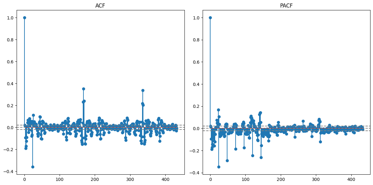
After applying the seasonal differencing, the time series looks much more stationary, and the strong 24-hour seasonality in the ACF has been significantly reduced. But we can still see the weekly seasonality so lets remove the weekly seasonality in the same way as 24-hour seasonality.

ADF Test:
----------------------------------------
ADF Statistic: -26.2230
p-value: 0.0000
Critical Value 1%: -3.4311
Critical Value 5%: -2.8619
Critical Value 10%: -2.5670
----------------------------------------

KPSS Test:
----------------------------------------
KPSS Statistic: 0.0905
p-value: 0.1000
Critical Value 10%: 0.3470
Critical Value 5%: 0.4630
Critical Value 2.5%: 0.5740
Critical Value 1%: 0.7390
----------------------------------------

Stationarity Assessment:
The time series is stationary.

After applying the seasonal differencing, the strong 7-day seasonality in the ACF has been significantly reduced. In summary, clear daily and weekly seasonality suggests that certain times of the day and week consistently see higher or lower transaction rates.

Conclusion from EDA

• Client Behavior:

  • A majority of clients have a few transactions, but there's a segment with very high transaction frequency, possibly commercial users.
  • Flagging a station as 'favorite' shows a mild correlation with both increased transaction amounts and frequency.
  • The average distance clients travel to refuel varies. While many opt for stations closer to their residences, a notable proportion doesn't mind traveling further distances. This could be influenced by various factors such as brand preference, fuel quality, pricing, or different kind of users especially commercial truckers.

• Payment Amounts:

  • There's a consistent pattern in payment amounts, with smaller transactions being more common. However, the frequency of transactions does vary based on the month, day of the week, and hour of the day.

• Temporal Trends:

  • Transaction rates present daily and weekly patterns, with pronounced spikes observed around 14 to 17 o'clock and particularly on Fridays.